INTRODUCTION

Migration is an adaptive strategy of many animals to find more favorable conditions and increase probability of survival when habitat ranges are altered by climatic changes. Winter migration is driven by change in snow cover (Bennett and Tang, 2006; Sabine et al., 2002; Nicholson, Bowyer, and Kie, 1997). Low snow depth conditions are ideal for winter range because energy expenditure for travelling is minimized and there is a greater availability of winter forage (Nicholson, Bowyer and Kie, 1997; Bennett and Tang, 2006). Deep snow is associated with higher rates of mortality in migratory cervids (Bennett and Tang, 2006). Studies of cervid winter migration in North America have found that winter migration activities are triggered by exceeding certain snow depth thresholds. Sabine et al. (2002) found that the peak of white-tailed deer migration in northern regions of New Brunswick coincided with 40cm of snow accumulation, and that 76% of migrations observed occurred within two weeks of exceeding this threshold. Mysterud (1999) found that the latest migration of roe deer in Norway occurred when permanent snow cover reached a depth of 50 cm.

Studies on migratory patterns of cervids have focused mainly on small study areas, capturing only the home and migratory ranges of specific populations (Nicholson, Bowyer and Kie, 1997; Bennett and Wang, 2006; Mysterud, 1999; Sawyer, Lindzey and McWhirter, 2005; Sabine et al., 2002). The availability of snow water equivalent (SWE) data, a proxy for snow depth, across all the Canadian prairie provinces provides an opportunity for a regional-scale multi-species study on cervid migration. SWE is a more suitable parameter for analysis than snow depth because water content differs between the same depths of snow at different times of the winter season and changes in SWE are more indicative of snow melt, as a decrease in snow depth measurement may represent snowpack settlement rather than snow melt (Farnes, 2013). The prairie ecozone of Saskatchewan, Alberta, and Manitoba provides habitat for multiple cervid species: pronghorn antelope, whitetail deer, mule deer, elk and moose (Ecological Framework of Canada, n.d.).

Environment Canada has snow water equivalent (SWE) measurements collected in discrete locations across the Canadian prairie provinces. However, this dataset is sparsely distributed and discrete, making it unsuitable for observing fine-scale spatial patterns of snow distribution necessary for migration analysis (Bennett and Tang, 2006). Snow cover can be extremely variable across a large landscape due to variability in environmental factors such as topography, wind, and vegetation cover (Luo, Taylor and Parker, 2007). Since migration activities are triggered by surpassing a specific snow depth threshold, in order to predict winter migratory patterns, models of continuous snow coverage are needed. To create continuous data surfaces of SWE cover, spatial analysis was used to interpolate SWE point data.

Advancements in geostatistical methods allow for spatial interpolation to be performed over large-scale landscapes (Kondoh, Koizumi and Ikeda, 2013). Geostatistics is a branch of statistics that is concerned with spatially autocorrelated data and conducts analysis by incorporating spatial coordinates of all measurements (Olea, 2009; ESRI, n.d.a). The objective of geostatistics is to characterize spatial systems where there are unknowns. Geostatistical methods depend on a semivariogram, a plot of variability between known points over distance, to describe the relationship between known and unknown points and predict unknown values (Fraczek, Bytnerowicz and Arbaugh, 2001; Johnston et al., 2001). The use of the semivariogram as a predictor is dependent on Waldo Tobler’s First Law of Geography (GIS Geography, 2017) which states:

Everything is related to everything else, but near things are more related than distant things

This law informs the spatial statistical concept of spatial autocorrelation. Spatial autocorrelation is a type of spatial analysis that allows for measurement of similarities or differences between an object and other objects nearby. Positive spatial autocorrelation, or clustering, is when objects that are closer together are more similar, while negative spatial autocorrelation or dispersion is when objects that are closer together are more dissimilar (Legendre, 1993). Geostatistical interpolation assumes that naturally occurring spatial variation can be modelling with spatial autocorrelation (Johnston et al., 2001).

Spatial interpolation can also be done with deterministic methods, which only use mathematical techniques and not statistical ones to perform interpolation (Johnston et al., 2001). Geostatistical methods are considered to be more sophisticated, but also more complex while deterministic methods are simpler, but may be unsuitable for datasets where spatial relationships are unable to accurately described with mathematical formulas. For this study, four different interpolation methods are evaluated: Triangulated Irregular Network (TIN), Inverse Distance Weighting (IDW), kriging, and trend surface analysis. It is critical to identify the most appropriate spatial interpolation method as there is no ideal method, and suitability is based on study objectives, and the characteristics of the dataset used (Lu and Wong, 2008). The objective of this study is to assess four different methods of deterministic and geostatistical spatial interpolation methods to evaluate the suitability of different methods for interpolating continuous SWE surfaces.

METHODS

Data Description

A point dataset of SWE data from 1979 to 2004 was obtained from Environment Canada as a shapefile. The dataset contains 500 discrete SWE measurements that were collected approximately every five years and encompasses areas of the Northwest Territories, Alberta, Saskatchewan, Manitoba and the United States (Fig. 1). The method of data collection was not provided but SWE approximations are often derived from passive microwave satellite data (Canadian Cryospheric Information Network, 2015). Measurements are available from years 1979, 1984, 1990, 1995, 2000 and 2004. The SWE data uses transverse mercator North American Datum 1983 (NAD83) projected coordinate system and this data is located within the UTM Zone 12 N. The geographic coordinate systems is North American 1983. To perform spatial interpolation methods, the 1995 SWE dataset was selected for the use of this study.

Additional shapefiles of provincial and ecozone boundaries were retrieved from Statistics Canada and Canada Soil Information Service to provide spatial context for surfaces and to generate boundaries for the region of study interest.

Figure 1. SWE data covers the prairie provinces of Alberta, Saskatchewan, and Manitoba, as well as sections of the Northwest Territories, British Columbia and the USA.

Study Area

The focus of this study is on migration of cervid species in the Canadian prairies. The study area was delineated to isolate visuals to only the three prairie provinces (Fig. 2). The Prairies Ecozone are part of the Canadian Interior Plains, which are an extension of the Great Plains of North America (Ecological Framework of Canada, n.d.). This ecozone covers an area of 520 000 km2 and is one of the most altered areas of Canada as a result of intensive human activity such as resource extraction and agriculture. The region is also home to various cervid species including: pronghorn antelope, whitetail deer, mule deer, elk and moose (Ecological Framework of Canada, n.d.). The climate in the Prairie ecozone ranges from subhumid to semi-arid climate with mean winter temperatures of -18.3°C to -9.4°C and mean summer temperatures of 16.1°C to 19.7°C. Annual precipitation in the Prairie Ecozone is extremely variable, ranging from 250 mm in the arid grasslands to 700 mm in warmer, humid regions (Ecological Framework of Canada, n.d.) The ecozone is also characterized by prevalent high wind speeds, which ranges from 18-20 km hr -1 (Ecological Framework of Canada, n.d.).

It should be noted that while the focus is on cervids within the prairies, the prairie provinces encompass multiple terrestrial ecozones: Montane Cordillera, Taiga Plains, Boreal Plains, Taiga Shield, Boreal Shield, Hudson Plains, and Prairies, which will also be discussed (Fig. 3).

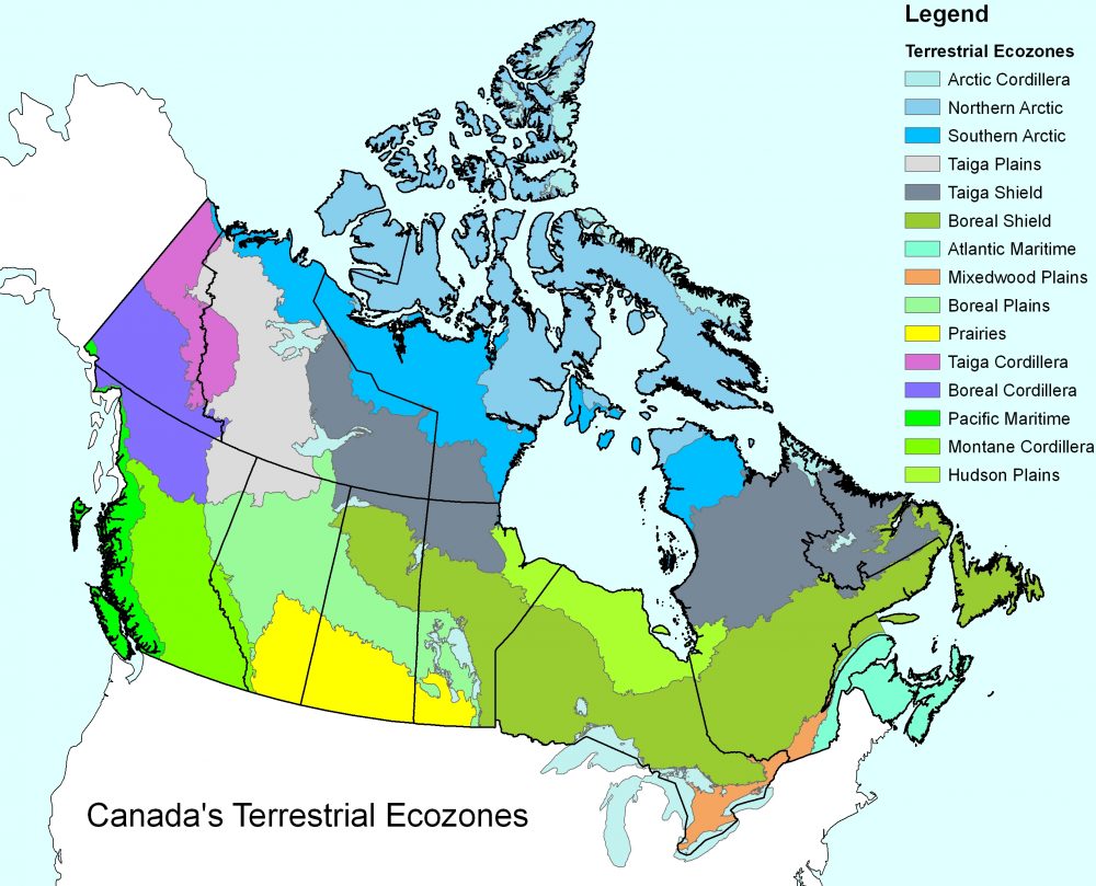
Figure 3. Terrestrial ecozones of Canada (Natural Resources Canada, 2017).

Data Visualization

Identifying the most appropriate method is critical to spatial interpolation because not all methods are appropriate for certain datasets (Lu and Wong, 2008). Visualizing data and understanding the characteristics of data distribution allows users to choose the most suitable spatial interpolation methods. Data visualization was explored through the use of histograms, trend analysis plots, QQ plots, and semivariogram clouds. These visualization tools were used to assess the spatial autocorrelation patterns that exist within the SWE dataset and understand the overall distribution of SWE measurements in the 1995 measurement year.

The histogram was used as the first method of data visualization, which showed how the frequency distribution of measured SWE values based on predetermined bin sizes. The histogram provided statistical details on minimum and maximum SWE values, standard deviation, skewness, kurtosis, measures of central tendency, and quartile values.

A Normal QQ Plot was used to visualize the distribution of the SWE dataset over normal values. To accomplish this a graph of the distribution of SWE dataset is generated and plotted with a graph of standard normal distribution based on pairing of quantiles. The purpose of the QQ Plot is to demonstrate which data points in the 1995 SWE dataset are normally distributed and which data points are not. Where the distribution of SWE data deviates from the linear regression normal line represents areas where data is not normally distributed.

The trend analysis plot is one of the most useful data visualization and exploration tools used because it allows data to be visualized in three dimensions, with north-south and east-west on the x and y-axis and point values on the z-axis. This visualization tool was used to explore the 1995 data set and was used to identify directional trends which were subsequently accounted for during interpolation.

The semivariogram cloud can be used to explore data as well as prepare for kriging interpolation, which is dependent on semivariogram modeling to calculate unknown values. The semivariogram cloud allows spatial autocorrelation between measured points to be examined with variance is plotted on the y-axis and the distance between points in plotted on the x-axis. The semivariogram contains three important components: (1) range, (2) sill, and (3) nugget (Fig. 4). The lag distance where variability begins to flatten is the range and it signifies that past that distance no spatial autocorrelation exists.The sill is the variance value at the range and typically represents the maximum value of variability. Points that have lower values on the y-axis are more similar (Johnston et al., 2001).

The nugget is the y-intercept, and should ideally be zero. When the nugget is above zero, the cause may be measurement error resulting from systematic error, random error, or blunders. The nugget may also be greater than zero as a result of variation at distances smaller than the sampling interval (Johnston et al., 2001). Selection of lag size is important in using the semivariogram because when bins are too large short-range autocorrelation that exists may not be noticeable while bins that are too small will have too few points to derive a representative bin average (Johnstone et al., 2001).

Figure 4. Semivariogram components (ESRI, n.d.a)

An average nearest neighbor tool was used to generate nearest neighbor values for the SWE data to be an estimated lag size for interpolation as well as exploring semivariograms. An omnidirectional semivariogram cloud was generated first and used to explore where high and low spatial autocorrelation existed in the prairie ecozone by highlighting different regions of the semivariogram cloud. The omnidirectional semivariogram was generated initially using a lag size of 34.4 km, which was the calculated average nearest neighbor, but the size was determined to be too small and unable to represent the entire surface extent. The lag size and number of lags were continually increased and adjusted to identify a size able to represent the surface entirely of 120 km and 16 lags.

A directional semivariogram cloud was generated using the same lag size and number of lags to identify the existence of directional trends in the data. Angle directions were chosen based on previously inferred trends derived from the trend analysis plot as well as from the semivariogram surface visualization provided in the omnidirectional semivariogram. Angle tolerance and bandwidth settings for search directions were kept at the default settings. The directional semivariogram search results were recorded to inform proceeding spatial interpolation methods used.

Interpolation Methods

In preparation for beginning interpolation, the SWE dataset was divided into a training set used to produce surfaces and a testing set to validate surfaces. Data subsetting was done at random to allow for unbiased distribution of data points between the training and testing dataset. Data subsetting can be performed through GIS software or statistical software based on user experience or preference.

Triangulated Irregular Network

TIN is the simplest method of spatial interpolation and uses Delaunay triangulation to create a continuous surface from point data by generating triangles of nearest neighbor points (QGIS, n.d.). Each known point is attached by lines to the two closest vertices and triangles are delineated to have similar areas. Delaunay triangulation delineates triangles by drawing a circle around triangle vertices and assessing whether other vertices from other triangles are contained within the circle. The most suitable triangle can be encaptured by a circle without containing the vertices of other triangle. A mean value of the three known vertices of the triangle is calculated to give each triangle a value. No other user decisions were made because TIN does not have parameters to modify.

A TIN surface was automated using the SWE training dataset as an input. To validate the TIN, a raster layer was generated from the TIN, and then raster values were extracted to points using the SWE testing dataset and TIN raster as inputs. To calculate error in TIN interpolation, a value field was created to subtract observed raster values from real SWE values and visualized as points using a graduated color symbology to identify distribution of high and low error values across the TIN surface.

Inverse Distance Weighting

IDW is a commonly used deterministic method of spatial interpolation that is simple to use because of the minimal parameter input and computational requirements (Lu and Wong, 2008). IDW assumes that any pair of points has a relationship that is inversely related to the distance between two points. The influence of known values on unknown values diminishes over distance (Luo, Taylor and Parker, 2007). A power function is applied to take into consideration that this assumption is not uniform, and will modify distance weights. With a power function of zero there is no decrease in weight as distance increases, and as the power function increases, the decrease in weight over distance is more rapid. Larger power function values result in surfaces that are less smooth as a result of greater local influence. The value of the power function is a parameter that can be modified by users. The user is also able to define the search neighborhood. Parameters that can be assigned in the search neighborhood are: neighborhood shape, neighborhood size, search orientation, maximum number of neighbors, and minimum number of neighbors

Generation of IDW surface was done with the full SWE dataset to maximize the known value points used to interpolate unknown values. The power function value was optimized automatically based on the SWE dataset. A 34 km radius was used to find neighbors, based on mean nearest neighbor distance. Cross-validation was used to identify the difference between observed and original SWE values at known points and generate error as a point layer.

Trend Surface Analysis

Global and local polynomial interpolation or deterministic spatial interpolation method, which create a continuous surface by creating a floating point grid using polynomial regression (Sheikhhasan, 2006). Global and local polynomial interpolation can be used to generate continuous surfaces by fitting different order polynomials to data trends (ESRI, n.d.c). The global polynomial interpolation allows users to generate one polynomial function up to the tenth order to generate a surface characterizing large-scale global trends in data, and is most suitable for datasets where variation over space is slow. Comparatively, a local polynomial interpolation allows users to generate multiple polynomial functions to fit to the dataset, and is most suitable for identifying short-range variation. The local polynomial interpolation also has a selection of general and advanced parameters that can be modified based on user preference and experience. A noteworthy parameter of local polynomial interpolation is exploratory trend surface analysis, which allows users to analyze trends before detrending occurs and is able to modify other parameters such as bandwidth and search neighborhood properties.

For the purpose of this study, global and local polynomial methods were used for trend surface analysis to identify the location of global and local trends and remove them from the dataset to generate more accurate surface layers. This allows the local and global polynomial interpolation methods to aid in the original data exploration portion of the study by finding tendencies of sample data as well as be used to generate their own continuous surface layers.

Each order of polynomial was tested for global polynomial interpolation to assess how mean error and RMSE changes as polynomial order changed. The most suitable global polynomial interpolation was selected based on previous data exploration and observations on data trends. Cross-validation was used to identify the difference between observed and original SWE values at known points and generate error as a point layer.

A second order polynomial was used for local polynomial interpolation selected because data exploration done using trend analysis plot and semivariogram cloud. Based on the regular distribution of data and order of polynomial, quartic kernel was selected (ESRI, n.d.d). Other model parameters were optimized based on this input.

Kriging

Kriging is a commonly used geostatistical method of spatial interpolation in environmental and wildlife modelling to create distribution and abundance maps from point data, and is considered one of the most sophisticated geostatistical methods (Kondoh, Koizumi and Ikeda, 2013; Fraczek, Bytnerowicz and Arbaugh, 2001). An advantage that is offered by kriging is that it is an appropriate method for interpolating point data sets that are irregularly arranged (Kondoh, Koizumi and Ikeda, 2013). Kriging interpolates unknowns and describes the relationship between known and unknown points by using a semivariogram, which shows the pattern in variance between points over distance (Fraczek, Bytnerowicz and Arbaugh, 2001). The semivariogram allows users to explore the relationship between distance and, as kriging assumes that closer points will be more similar (Kondoh, Koizumi and Ikeda, 2013).

To determine a value at an unknown point kriging gives a weight to all known points based on their relationship to the unknown point. The assignment of weights in kriging and the calculation of unknown points are based on modelling the semivariance. Choosing a model to fit the empirical semivariogram is one of the most important user-selected parameters of kriging interpolation. The important characteristics considered while choosing a model was the behavior of variance of the origin and the behavior of variance approaching the sill.

There are many types of kriging interpolation available which have different assumptions and suitability depending on data. Types of kriging include: ordinary, simple, universal, indicator, probability, disjunctive, empirical bayesian and areal interpolation. For this study only ordinary kriging was used for spatial interpolation of SWE data (Fig. 5). The assumptions made by ordinary kriging are (Olea, 2009):

Mean is constant but unknown
There is no underlying spatial trend in data
Surface is isotropic
The properties of the semivariogram are definable
The same variogram applies for the entire study area

Ordinary kriging was formulated as an improved version of simple kriging, which assumes a known and constant mean, which makes it a more restrictive kriging method than ordinary kriging (Olea, 2009). The objective of ordinary kriging is to identify optimal weights to minimize mean square error.

Figure 5. Formula for ordinary kriging spatial interpolation (Olea, 2009).

Since kriging assumes no global or local trends, all trends must be removed before fitting a semivariogram model. Global trend removal was done by selecting a constant, first, second, or third order of trend removal and selecting or optimizing properties automatically similar to the process of local polynomial interpolation. Second degree trend removal was used and properties were optimized based on a quartic kernel based on the trend identified through semivariogram cloud and trend analysis plot exploration as well as local polynomial interpolation trend surface analysis.Directional trend removal was performed based on directional semivariogram cloud exploration and visualization of the semivariogram map. A spherical model was selected based on the characteristics of the empirical semivariogram (Fig. 6).

Figure 6. Spherical model fitted to empirical semivariogram of SWE data during kriging interpolation.

RESULTS

Data Visualization

Data visualization and exploration methods demonstrated that the 1995 SWE dataset does not exemplify a normal distribution (Fig. 7). The majority of SWE values are 0-114 mm with the highest frequency of SWE points being within the 0-29 mm, 29-57 mm and 57-86 mm ranges, in declining frequency. The maximum SWE value is 286 mm and the spatial distribution of SWE values between 86 mm and 286 mm are mainly outside of the prairie ecozone boundaries or along the perimeters (Fig. 8). SWE values are higher in the east and the north and most variation from normal distribution are a result of lower than standard normal value SWE points in the southwest part of the prairie ecozone (Fig. 8).

Figure 8. Spatial distribution of high value and low value SWE data points from the 1995 dataset as discovered through histogram and QQplot data visualization

The omnidirectional semivariogram cloud (Fig. 9) was generated using the identified lag distance of 120 km and 16 total lags. Each red dot on the semivariogram cloud is representative of the relationship between a pair of known points from the SWE dataset. A dataset with positive autocorrelation would have a higher frequency of points in the upper-left of the semivariogram cloud which would diminish toward the right, indicating that the relationship between points is reduced by distance. The omnidirectional semivariogram cloud demonstrates that there is high and low variability between points distributed relatively evenly across the 1995 SWE dataset. As seen in the histogram, QQ plot and trend analysis plot, variability within close points were found in the NE of the dataset, which is actually outside of the prairie ecozone.

Figure 9. Omnidirectional semivariogram cloud of 1995 SWE dataset visualizing the variability between points over distance.

The directional semivariogram cloud generated using a search direction of 110° or NE to SW (Fig. 10). The shape of the directional semivariogram cloud is indicative of positive spatial autocorrelation and fewer point relationships with high variability compared to the omnidirectional semivariogram, which is visualized by the fewer frequency of points on the semivariogram cloud at higher values on the y-axis.

Figure 10. Directional semivariogram cloud of 1995 SWE dataset visualizing the variability between points over distance with a NW to SE search direction.

Interpolation Methods

Continuous surfaces were generated for SWE data using IDW, kriging, trend surface analysis and TIN methods of spatial interpolation. The maximum and minimum values of each method was compared as a method of assessing model accuracy (Table 1). Cross-validation point layers were generated to determine error of interpolation at known values from the SWE dataset. Errors for each method of interpolation were also assembled as a method of comparing model accuracy (Table 2). Error values were derived from cross validation used to assess the performance of interpolation methods, which removes the known observations individually and uses the model to estimate values for it based on remaining observations

The mean error is the average difference between observed values and actual values, and a low mean error value that is close to zero shows that there is no bias in interpolation (ESRI, n.d.e; Luo, Taylor and Parker, 2007). The Root Mean Square Error (RMSE) is a measurement of how closely model predictions are to measured values and a lower value means more accurate interpolation. The average standardized error is the average of prediction standard errors. The mean standardized error is an average of the standardized error and should be close to zero if interpolation is accurate. The RMSE standardized should be a value close to one. If RMSE standardized is greater than one than the interpolation method underestimated the variability of data values and if the RMSE standardized is less than one than the interpolation method overestimated the variability of data values. RMSE and average standardized error should be similar (ESRI, n.d.e).

Table 1. Minimum and Maximum values (mm) of observed SWE data and different spatial interpolation methods.

Table 2. Error values for interpolation methods used to generate continuous SWE surfaces.

Triangulated Irregular Network

The TIN surface generated contained continuous values for the entire prairie ecozone, but was unable to interpolate values for parts of northern Saskatchewan and Manitoba where SWE data values were limited (Fig. 11). The range of TIN values ranges from 0 to 285.7 mm, reflecting the same value range as the original SWE dataset. SWE values highest in northern Alberta in the Taiga Plains ecozone and the northeastern border of the boreal shield ecozone in Saskatchewan. Within the prairie ecozone SWE values are lower in southern Alberta and southwestern and southcentral Saskatchewan. SWE values in the prairie ecozone are the highest near the boundary of the Boreal Plain ecozone and in southeastern Saskatchewan near the Manitoba border. The TIN validation point layer generated from the SWE test data subset identifies the error of interpolated points at locations with known value points. Lower error is identified by purple and green points while higher error is identified by white, yellow, and brown points. Regions of higher error are distributed across the study area with limited clustering. Error values range from -39 to 256 mm.

Figure 11. Interpolated TIN surface of 1995 SWE dataset.

Figure 12. Error of TIN interpolation at known values of 1995 SWE dataset.

Inverse Distance Weighting

The IDW surface covers the entire area of the prairie provinces except for the eastern tip of Manitoba (Fig. 13). IDW interpolated SWE values range from 0 to 192.8 mm. The area of highest SWE values based on IDW is in the Taiga Plain region of northern Alberta. WIthin the prairie ecozone the highest SWE values are within the 69.4 to 97.4 mm class. The lowest interpolated SWE values are in southern Alberta and southeast to southcentral Saskatchewan. Cross-validation revealed the distribution of interpolation error of IDW to be distributed relatively evenly across the prairie provinces, but with some clustering (Fig. 14). Error is lowest at green and yellow points with higher error in white, purple and brown points. Purple values are most prevalent near the border between the Prairie and Boreal Plain ecozone and in southern Saskatchewan. Error values range from -147.6 to 71.2 mm.

Figure 13. Interpolated IDW surface of 1995 SWE dataset.

Figure 14. Error of IDW interpolation at known values of 1995 SWE dataset.

Trend Surface Analysis

Global Polynomial Interpolation

The global polynomial interpolation method was able to generate a surface that covers the entire region of the prairie provinces except for the eastern tip of Manitoba, which is the same spatial coverage as IDW interpolation (Fig. 15). SWE values range from -67.6 to 109.9 mm based on global polynomial interpolation. Distribution of SWE data values across the surface are extremely smooth with limited local variation as a result of being a global method. SWE values are lowest in southern Alberta and southwestern and southcentral Saskatchewan and highest in northeastern Saskatchewan and northern Manitoba. WIthin the Prairie ecozone SWE values are highest in the upper boundaries of the ecozone in Alberta and Saskatchewan as well as in the southwestern region of Manitoba. Cross-validation of global polynomial interpolation shows that error values range from -108.7 to 91.2 mm and the areas of lowest error are visualized by green and yellow points (Fig. 16).. White, purple and brown points indicate areas of greater error. Error clustering is found between the border of the Boreal Plain and Prairie ecozones, particularly in Alberta and Saskatchewan. There is also some clustering occurring in multiple areas in the Boreal Shield ecozone in Saskatchewan and Manitoba. Error is lowest in areas with smaller SWE values identified by blue to green classes.

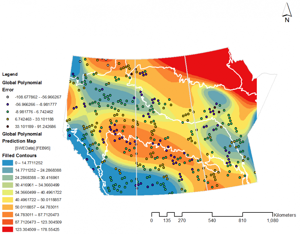
Figure 16. Error of global polynomial interpolation at known values of 1995 SWE dataset.

Local Polynomial Interpolation

The local polynomial interpolation method was able to interpolate values for all of Alberta, but unable to generate values for areas of northern Saskatchewan and Manitoba (Fig. 17). SWE data values are highest in northern Alberta and regions of the Boreal Shield in parts of Saskatchewan and Manitoba. The range of interpolated SWE values based on local polynomial interpolation were -12.0 to 155.1 mm. Within the Prairie ecozone SWE values are highest at the northern boundary near the Boreal Plain in Alberta and Saskatchewan, and there are also higher values observed in the southern border between Saskatchewan and Manitoba. Lowest values are observed in southern Alberta and southwestern and southcentral Saskatchewan. Cross-validation of local polynomial interpolation error revealed that error was well distributed with limited areas of clustering (Fig. 18). Error values ranged from -144.4 to 80.3 mm with the lowest error being represented by green points followed by yellow points. Higher areas of error were represented by white, yellow and brown points. Higher error was more commonly found in areas with higher SWE values, while lower SWE values such as the ones found in southern Alberta and Saskatchewan were mainly associated with low error green points.

Figure 18. Error of local polynomial interpolation at known values of 1995 SWE dataset.

Kriging

Kriging interpolation created a surface that covered the entire region of the prairie provinces except a small northeastern portion of Manitoba (Fig. 19). SWE values based on kriging interpolation ranged from -2.0 to 211.1 mm. Lowest SWE values were found in southern Alberta and southwest and southcentral Saskatchewan. Highest SWE values were found in small centralized regions of northern Alberta, northern Saskatchewan, and northern Alberta. The highest SWE data values interpolated in the Prairie ecozone are along the boundary with the Boreal Plain ecozone in Alberta and Saskatchewan as well as in the southern border of Saskatchewan and Manitoba. Lowest SWE values within the Prairie ecozone are the same as lowest SWE values across the prairie provinces. Cross validation showed that kriging interpolation error ranged from -128.8 to 85.3 mm (Fig. 20). The lowest error is classified by green points and followed by yellow points. White, yellow and brown points are indicative of regions of higher error. Error clustering is limited within the kriging surface. A small cluster of purple-class error points are found near the Boreal Shield and Boreal Plain boundary of central Manitoba. Other higher value error points found on the kriging surface are shown to be distributed across the surface and not clustered in regions of high error.

Figure 20. Error of kriging interpolation at known values of 1995 SWE dataset.

DISCUSSION

SWE data was found to be widely variable across the prairie provinces of Alberta, Saskatchewan, and Manitoba. Due to the extremely spatially variable nature of SWE, points measurements may not be an adequate method of characterizing snow cover (Erxleben, Elder and Davis, 2002). Additionally, manual collection of SWE measurements in remote regions can be both time and resource intensive, which is why spatial interpolation offers an opportunity to utilize SWE point data to generate usable tools. The distribution of the 1995 SWE dataset demonstrated that SWE data is not normally distributed and that both global and local trends existed within the data. The data collection region of the 1995 SWE dataset covers multiple terrestrial ecozones marked by different compositions of climate regimes, vegetation, and environmental influences. Variations in SWE values can be a result of such environmental influences including atmospheric circulation patterns and topography (Harshburger et al., 2010; Derksen et al., 2000). Due to the complexity in snow cover and the environmental factors that influence snow cover distribution, SWE values can be difficult to interpolate (Erxleben, Elder and Davis, 2002).

REFERENCES

Bennett, D., and Tang, W. (2006). Modelling adaptive, spatially aware, and mobile agents: Elk migration in Yellowstone. International Journal of Geographical Information Science, 20(9), 1039-1066. DOI: 10.1080/13658810600830806
Canadian Cryospheric Information Network. (2015, June 4). Snow Water Equivalent. Retrieved from https://www.ccin.ca/home/ccw/snow/current/swe
Ecological Framework of Canada. (n.d.). Prairie Ecozones. Retrieved from http://ecozones.ca/english/zone/Prairies/index.html
Erxleben, J., Elder, K., and David, R. (2002). COmparison of spatial interpolation methods for estimating snow distributions in the Colorado Rocky Mountains. Hydrological Processes, 16, 3627-3649. DOI: 10.1002/hyp.1239
ESRI. (n.d.a). What is geostatistics. ArcGIS Pro. Retrieved from http://pro.arcgis.com/en/pro-app/help/analysis/geostatistical-analyst/what-is-geostatistics-.htm
ESRI. (n.d.b). A quick tour of Geostatistical Analyst. ArcMap. Retrieved from http://desktop.arcgis.com/en/arcmap/latest/extensions/geostatistical-analyst/a-quick-tour-of-geostatistical-analyst.htm
ESRI. (n.d.c). How global polynomial interpolation works. ArcGIS Pro. Retrieved from http://pro.arcgis.com/en/pro-app/help/analysis/geostatistical-analyst/how-global-polynomial-interpolation-works.htm
ESRI. (n.d.d). How local polynomial interpolation works. ArcGIS Pro. Retrieved from http://pro.arcgis.com/en/pro-app/help/analysis/geostatistical-analyst/how-local-polynomial-interpolation-works.htm
ESRI. (n.d.e). Cross Validation. ArcGIS Pro. Retrieved from http://pro.arcgis.com/en/pro-app/tool-reference/geostatistical-analyst/cross-validation.htm
Derksen, C., LeDrew, E., Walker, A., and Goodison, B. (2000). Winter season variability in North American Prairie SWE distribution and atmospheric circulation. Hydrological Processes, 14, 3273-3290. DOI: 10.1002/1099-1085(20001230)14:18<3273::AID-HYP203>3.0.CO;2-W
Farnes, P. (2013). Estimating Snow Water Equivalent at NWS Climatological Stations. Paper presented at 81st Annual Western Snow Conference, Jackson Hole, WY. Retrieved from https://westernsnowconference.org/sites/westernsnowconference.org/PDFs/2013Farnes.pdf
Frassnacht S., Dressler, K., and Bales, R. (2003). Snow water equivalent interpolation for the Colorado River Basin from snow telemetry (SNOTEL) data. Water Resources Research, 39(8), 1208. DOI: 10.1029/2002WE001512
Fraczek, W., Bytnerowicz, A. and Arbaugh, M. (2001) Application of the ESRI Geostatistical Analyst for Determing the Adequacy and Sample Size Requirements of Ozone DIstribution Models in the Carpathian and Sierra Nevada Mountains. The Scientific World Journal, 1, 836-854. DOI: 10.1100/tsw.2001.317
Huang, C., Wang, H, and Hou, J. (2015). Estimating spatial distribution of daily snow depth with kriging methods: combination of MODIS snow cover area data and ground-based observations. The Cryosphere Discussion, 9, 4997-5020. DOI: 10.5194/tcd-9-4997-2015.
Harshburger, B., Humes, K., Walden, V., Blandford, T., Moore, B., and Dezzani, R. (2010). Spatial interpolation of snow water equivalency using surface observations and remotely sensed images of snow-covered area. Hydrological Processes, 24, 1285-1295. DOI: 10.1002/hyp.7590
Johnston, K., Ver Hoef, J., Krivoruchko, K. and Lucas, N. (2001). Using ArcGIS geostatistcal analyst. Redlands, CA: ESRI.
Kondoh, H., Koizumi, T. Ikeda, K. (2013). A geostatistical approach to spatial density distributions of sika deer (Cirvus nippon). Journal of Forest Research, 18(1), 93-100. DOI: 10.1007/s10310-011-0326-x
Legendre, P. (1993). Spatial Autocorrelation: Trouble or New Paradigm. Ecology, 74(6), 1659-1673. DOI: 10.2307/1939924
Lu, G., and Wong, D. (2008). An adaptive inverse-distance weighting spatial interpolation technique. Computers and Geosciences, 34(9), 1044-1055. DOI: 10.1016/j.cageo.2007.07.010
Luo, W., Taylor, M., and Parker, S. (2007). A comparison of spatial interpolation methods to estimate continuous wind speed surfaces uses irregularly distributed data from England and Wales. International Journal of Climatology, 28, 947-959. DOI: 10.1002/joc.1583
Mysterud, A. (1999). Seasonal migration pattern and home range of roe deer (Capreolus capreolus) in an altitudinal gradient in southern Norway. Journal of Zoology, 247(4), 479-486.
Natural Resources Canada. (2017). Forest classification. Government of Canada. Retrieved from http://www.nrcan.gc.ca/forests/measuring-reporting/classification/13179
Nicholson, M., Bowyer, R., and Kie, J. (1997). Habitat Selection and Survival of Mule Deer; Tradeoffs Associated with Migration. Journal of Mammalogy, 78(2), 483-504. DOI: 10.2307/1382900
Olea, R. (2009). A Practical Primer on Geostatistics. Reston, VA: United States Geological Survey. Retrieved from http://citeseerx.ist.psu.edu/viewdoc/download?doi=10.1.1.593.85&rep=rep1&type=pdf
QGIS. (n.d.) Spatial Analysis (Interpolation). Retrieved from https://docs.qgis.org/2.2/en/docs/gentle_gis_introduction/spatial_analysis_interpolation.html
Sheikhhasan, H. (2006). A Comparison of Interpolation Techniques for Spatial Data Prediction (Master’s thesis). Retrieved from https://staff.fnwi.uva.nl/a.s.z.belloum/MSctheses/Hamzeh_C.pdf
Sabine, D., Morrison, S., Whitlaw, H., Ballard, W., Forbes, G. and Bowman, J. (2002). Migration Behavior of White-Tailed Deer under Varying WInter CLimate Regimes in New Brunswick. The Journal of Wildlife Management, 66(3), 718-728. DOI: 10.2307/3803137
Sawyer, H., Lindzey, F., and McWhirter, D. (2005). Mule deer and pronghorn migration in western Wyoming. Wildlife Society Bulletin, 33(4), 1266-1273. DOI: 10.2193/0091-7648(2005)33[1266:MDAPMI]2.0.CO;2